PRISM CCD testing data reduction package user manual

---

This user manual is intended to explain how the images have to be acquired and processed with the PRISM's CCD testing package.

Those procedures are used at ESO in order to characterize CCD cameras before being installed to the telescope or for CCD preliminary testing.

For a given test, requiring many images, they ALL must have the same amount of pixels (i.e. width/height) and being the same data file type (i.e.: integer or floating point data). Mixtures of image seize and/or data type will result directly in a failure.

1. Non-Linearity and Conversion Factor (e-/ADU)

This measurement is used to get the conversion factor (e-/ADUs) and the CCD linearity.

The CCD must be illuminated by a very stable light source, the resulting image has to be as "flat" as possible.

10 couples of images, at least, must be acquired  with different exposure times, ranging from the full dynamic (intrinsic CCD dynamic or Analog to Converter dynamic) to the bias level.

For instance : (16 bit camera ranging from 0 to 65535 ADU)

Take at least 16 couples of images and try to achieve up to 95% of saturation level, to explore the all range.

Avoid to take images with increasing or decreasing exposure times as for instance 2,5,10,50 sec, use instead a random order as 2,50,10,5 sec.

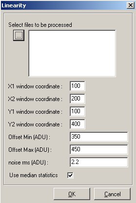
When the PRISM software dialog box pops up, you have to enter a window where the stats will be achieved (X1,X2,Y1,Y2). Keep in mind not to include defects in this window. The statistic can be either "median" or "classic" type. Set the "median" to avoid the effect of out of range or defective pixels, median is less sensitive to local contaminants.

The range (offset min et max.), comes from the offset image mean. In that case supply : Offset/bias level min = Offset  -10% and Offset max= offset +10%), this allows to optimize the offset deviation effect with respect to shutter errors. To known this figure (Bias level), you have to measure it form a set of bias images.

!! Multiples files can be selected by keeping the ALT key down while selecting files in the open dialog box !!

PRISM software compute automatically the conversion gain in  e-/ADU and the residual non-linearity expressed in % units, using the whole double exposure set of images. A photon-transfer curve is plotted as an output.

Results

Console output :
Optimum offset(ADU) (1): 368
Non linearity (Peak to peak) :  (1): 0.4367% / -0.8695%
Optimum offset(ADU) (2): 368
Non linearity (Peak to peak) :  (2): 0.3741% / -0.1807%
Conversion factor  e-/ADU : 1.9926
-> RMS error : 0.12428
Readout noise (e-) : 4.7822
 

The data(1) uses the first set of images and data(2) the second set.

The following curves are displayed,  no need to make a table sheet for a plotter like Excel.

Linearity curve according to exposure time.

Residual non linearity curve

Photon transfer curve, this plot is used to compute the conversion factor (e-/ADU).

Method used : see reference

VERY IMPORTANT : be aware that FITS files are coded sometime as a true 16 bit data (0-65535). PRISM adapts data type according to the input file and to save memory space, but we recommend strongly to open the "Option/FITS options" menu, and to set the "Load 16bits unsigned FITS file to floating point data" as checked.

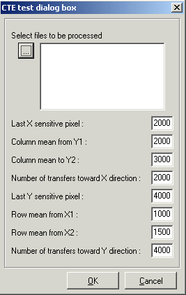
2. Charge transfer Efficiency (CTE) EPER method

This is the dialog box related to CTE measurement :

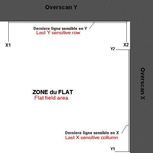
For this purpose, acquire a single flat field  image reaching 95% of the ADC dynamic range. The camera shall be able to read the array beyond the photosensitive area. This area beyond the image is called "OVERSCAN", and contains fake pixels having the bias value provided by the electronic readout chain and CCD. This area shall be extended both in X and Y directions. This kind of image has to be provided to PRISM software to compute CTE.

Y1,Y2 is the area to perform the mean of the last light sensitive row and the X1,X2 is the range to compute the last mean column. The number of transfer across  X and Y is typically the light sensitive image part.

Console output:
Loading :F:\Images\Frankie\CTE\Cte_0001
Mean -> Last X :58491.6583936574 Last X+1 :469.123061013444 Overscan area :449.922095829024
Horizontal CTE = 0.999999838470179 / 6 nines
Mean -> Last Y :65510.6978248089 Last Y+1 :495.093474426808 Overscan area :445.12810646144
Vertical CTE = 0.999999625037444 / 6 nines

References :
http://www.stsci.edu/instruments/acs/ctewg/papers/jones_fpr.pdf

3. Quantum efficiency and PRNU (Photo Response Non uniformity)

This is a really difficult measurement, because the result has to be provided in absolute figures, and you MUST have to input calibration data.

Basic knowledge regarding QE measurement must be known !!

The usual scheme is to use an absolute quantum efficiency calibrated photodiode installed at the same position as the CCD will be, and to use flat field images made in the front of an integrating sphere, fed by one or two  monochromators. This setting allows you to get different flat field images at different wavelengths and short bandwidth.

The incoming light wavelength is typically ranging from 300 to 1100 nm, with a short bandwidth, such as 5nm. The photodiode current is measured, and the photodiode manufacturer calibration curve enables you to compute the amount of photons per square centimeter and per second. This is an example of a photodiode calibration file (as a text file) :

# No TABS
# ratio bdw 4 # col 1 Wavelength
# col 2 Flux on the CCD surface, expressed in photons/sec/cm2
# col 3 Current that is measured at integrating sphere level or closeby to the CCD
320    1.1e+8   0.209e-9
340    2.55e+8  0.544e-9
360    5.18e+8  1.115e-9
380    9.27e+8  2.124e-9
400    1.44e+9  3.646e-9
450    2.9e+9   7.94e-9
500    3.54e+9  10.207e-9
550    3.9e+9   11.5e-9
600    3.97e+9  11.74e-9
650    3.6e+9   10.85e-9
700    3.09e+9  8.96e-9
750    2.35e+9  6.67e-9
800    1.54e+9  4.224e-9
850    1.66e+9  4.52e-9
900    1.42e+9  3.871e-9
950    3.4e+9   8.6e-9
1000   3.16e+9  7.65e-9
1100   2.42e+9  1.224e-9 Afterward, the optical transmission of the dewar window according to the wavelength as to be provided (as a text file).# Window transmission
# col 1 Wavelength
# col 2 Relative transmission
320    0.94
340    0.97
360    0.98
380    0.98
400    0.99
450    0.99
500    0.99
550    0.996
600    0.9856
650    0.9615
700    0.926
750    0.889
800    0.8517
850    0.8153
900    0.7873
950    0.7627
1000   0.7466
1100   0.723
 

IMPORTANT : For all the wavelengths used, calibration photodiode text file and window calibration transmission text file MUST match each other. It means that the same wavelengths must be entered in the two calibration files (Otherwise an error will occur). FITS files must include the following HEADER Keywords :

WAVLG = 550 // Central wavelength : Expressed in mn
BANDW = 5 // Bandwith : Expressed in mn
FLUX = 1.2E-5 // Photodiode current expressed in Amps
or
1_FLUX = 1.2E-5 // Photodiode current expressed in Amps

Regarding the CPA image file : if images have been acquired with PRISM, the previous figures are entered automatically into the CPA file header.

A reference offset/Bias image (resulting from a median stack of 10 offset/bias images) is mandatory, also the integration time must be limited in a way that the CCD dark current remains negligible.

Once having entered all the calibration files in the software dialog box, the analysis window  X1,X2,Y1,Y2 must be chosen in the way that it must not have any serious defects (black hole, bright pixels).

Conversion factor must have been measured previously (see method 1 or 2).

Distance during calibration/measurements allows the reference photodiode not to be at the same distance as the CCD, and to apply a 1/d^2 correction. This correct for few centimeters effects.

Results

This is the console output results, for each FITS files, it yields to :

Wavelength in nm ; Flux in Amps ; Exposure in sec ; Count values in e-
Filename         Wavelength  Flux       Exposure  Mean    Stddev.Rms  Median  Mean-Median
QE0002.fits      320         1.749E-10  180       21400   484.08      21400   -0.051972
QE0034.fits      340         4.754E-10  180       60662   1281.8      60678   -15.768
QE0004.fits      360         1.0234E-9  79.523    60965   1260.3      60976   -11.264
QE0032.fits      380         2.0072E-9  36.67     60579   832.35      60568   10.537
Qe0006.fits      400         3.5871E-9  20.472    60341   578.48      60342   -1.3613
QE0030.fits      450         8.4612E-9  9.223     60576   473.26      60582   -6.0853
QE0008.fits      500         1.1307E-8  7.248     60050   462.21      60052   -2.3795
QE0028.fits      550         1.3328E-8  6.904     64220   478.24      64226   -5.6408
QE0010.fits      600         1.4012E-8  6.438     59948   446.82      59952   -4.0484
QE0026.fits      650         1.3279E-8  7.296     59910   442.79      59914   -4.2144
QE0012.fits      700         1.1196E-8  9.48      59680   450.23      59686   -5.5382
QE0024.fits      750         8.4697E-9  14.39     59830   481.27      59838   -8.0172
QE0014.fits      800         5.4537E-9  27.831    59990   533.66      60004   -13.601
QE0022.fits      850         5.9775E-9  33.177    59951   508.76      59960   -9.061
QE0016.fits      900         5.1913E-9  58.056    59327   941.36      59162   165.3
Qe0020.fits      950         1.2662E-8  49.111    61606   2471.5      62156   -549.94
QE0018.fits      1000        1.0568E-8  171.99    62739   3667.6      64178   -1438.6
QE0036.fits      1100        1.7114E-9  180       1006    82.472      994     12.022

Image #1 Bandwidth :5
PhotoDiode calibration Bandwidth :4
Filename         Wav.  PRNU%      QE%       FDio/FDio.cal   Ph/pix/sec e-/pix/sec  %Wind
QE0002.fits      320   2.262      61.065    0.83684         207.12     118.89      94
QE0034.fits      340   2.1125     69.312    0.87389         501.4      337.1       97
QE0004.fits      360   2.0669     73.139    0.91787         1069.8     766.77      98
QE0032.fits      380   1.3742     85.51     0.94499         1971       1651.7      98
Qe0006.fits      400   0.95867    93.401    0.98385         3187.7     2947.5      99
QE0030.fits      450   0.7812     95.421    1.0656          6953.3     6568.6      99
QE0008.fits      500   0.76969    94.847    1.1078          8823.7     8285.3      99
QE0028.fits      550   0.74462    91.842    1.1589          10170      9302.7      99.6
QE0010.fits      600   0.7453     88.622    1.1935          10661      9312.2      98.56
QE0026.fits      650   0.73904    86.151    1.2239          9913.7     8211.9      96.15
QE0012.fits      700   0.75434    78.263    1.2496          8687.5     6296        92.6
QE0024.fits      750   0.8043     69.666    1.2698          6714.2     4158.3      88.9
QE0014.fits      800   0.88938    56.584    1.2911          4473.7     2156        85.17
QE0022.fits      850   0.8485     44.878    1.3225          4939.4     1807.3      81.53
QE0016.fits      900   1.5912     30.209    1.3411          4284.7     1019.1      78.73
QE0020.fits      950   3.9762     14.732    1.4724          11264      1265.6      76.27
QE0018.fits      1000  5.7147     5.0888    1.3814          9821.7     373.16      74.66
QE0036.fits      1100  8.297      0.10033   1.3982          7613.2     5.5222      72.3
 

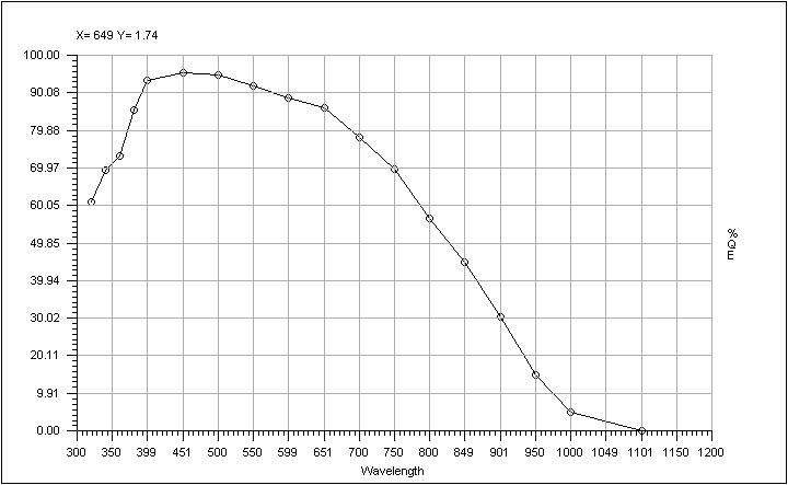
The PRISM software provides the quantum efficiency plot as following :

Also a PRNU curve is provided :

For instance, this is some images taken at different wavelength of the same area of the CCD (bandwidth=5nm and CCD EEV44 backside illuminated ) :

at 650 nm (very good uniformity)  

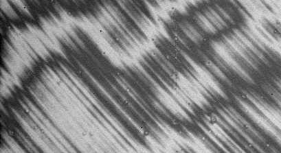
at 950 nm (nice fringing !)

Methods used :
The method employed here for QE is straightforward and based on the ratio between the amount of photon falling to the CCD surface for a given wavelength and the effective amount of photoelectrons read out at the output of the CCD. This is achieved by all the data coming from the calibration text files and figures found in the image file header, such as pixel size, exposure time, flux, wavelength, etc etc ...

The PRNU computes the histogram of the selected (X1,X2,Y1,Y2) area, and provide two figures : the intensities at 5% and 95% percentile. Let's call those figures Int1 and Int2, the PRNU is (Int2-Int1)/(Int1+Int2)*100%

4. Readout noise

The data acquisition process is straightforward : acquire at least five images in the total darkness having all zero sec exposure.

The input window X1,X2,Y1,Y2 is the window where the noise computation will take place. Take a window without any kind of defect and showing pure random noise (avoids hots pixels clusters).

Results :

The above curve is a stacked column mean over all the columns ,and allows you to display effect that would be drown or hidden by the readout noise .

To trace noise patterns, a Fast Fourier Transform (FFT) of the image is sometime recommended.

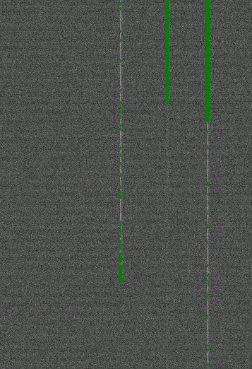
This image shows cosmetic defects (green cross) over a CCD bias image: these are pixels that are 5 sigma above the median noise + mean.

Console output:
Pixel amount taken to provide median frame :
noise0005 ->1  42.53%
noise0003 ->2  57.43%
noise0004 ->3  57.65%
noise0002 ->4  42.39%
Noise : 2.286 ± 0.005463 ADU
Pixel amount above 5 sigma : 17100 threshold (ADU) : 6.584

BEWARE : This measurement could be biased if care has not been taken concerning the file format.

Method used :
The RMS value is computed throughout the selected area. The final noise is the median noise from the set of the images. To trace bias defect, a median stack is performed to get rid of cosmic rays, and every pixel which is above or below five (5) sigmas is referenced as a bad pixel and mapped.

See also this

5. Dark current

As input image data, at least 3 images in total darkness has to be achieved, having the same exposure time for each (from 5 minutes to 2 hours depending on the cooling efficiency and CCD temperature).

A mean clean Offset or Bias  image MUST to be done as the result of the median stack of many individual bias frames. Also the conversion factor must be known accurately.

Be aware that sometimes residual image can disturb dark current measurement, especially if the CCD is cooled at -120C . Avoid to acquire the data just after having acquired high level flat fields. To watch this out : take ten dark frames at the same temperature and check whether or not the mean dark level is decreasing. Wipe the CCD many times before in the darkness. For instance take 10 darks exposure of one hour exposure, and do not use the first images (do not select the first four images).

As usual, the X1, X2, Y1, Y2 window is the window where the computation will be performed and must be clean of bright defects.

Results

This is the mean of all the columns sent to a single resulting column. The steps in the curves shows the defect induced by defect columns.. The same is displayed for the rows.

Here hots pixels map is provided. All pixels above 5 sigma noise+mean are shown and could be regarded as defects.

Console output:
Loading :F:\Images\Frankie\dark\run1@-120\dark0004.fits
Pixel size information NOT present or NULL in file header, so I take : 15 x 15(µm)
Loading :F:\Images\Frankie\dark\run1@-120\dark0003.fits
Loading :F:\Images\Frankie\dark\run1@-120\dark0002.fits
Loading :F:\Images\Frankie\dark\run1@-120\NoiseMedian.cpa
Integer data type...
Median search :
Compute median frame...
Pixel amount taken to provide median frame :
dark0004.fits ->1  27.92%
dark0003.fits ->2  44.71%
dark0002.fits ->3  27.37%
Offset -> Mean :327.1 Median : 327 ADU

Exposure time (s) =  1800
Dark current : 1.333 ± 0.4714 ADU
Dark current : 5.333 ± 1.886 e-/hour/pixel
Cosmic event rate : 1.195 ± 0.04297 events/min/cm²
Pixel amount above 5 sigmas : 10659 threshold (ADU) : 10.51
Dark current using median frame after median filtering : 5.128 e-/hour/pixel

Even, the software is able to provide the cosmic ray hit rate automatically.

Method used :
The software compute a median stack out of the N provided images and subtract the bias file to it. The dark current is the remaing amount of adus above the bias image (positive data). the defects are subtracted automatically as the difference between individual frames and the median stacked frame.

6. Linearity using TDI method

This method provides the same results as the classical method, the differences are the following :

• Only one image is necessary (whereas the other method requires many images and takes long time to be carried out).
• Absolutely insensitive to shutter errors.
• The output curve providing the residual non-linearity versus the measured signal is continuous  (whereas the other method provide discrete points)
• The measurement accuracy is much better than the one obtained by the classical different exposure method.
• Not limited by the PRNU of the CCD.

 

This method has, nevertheless, constraints, where the main drawbacks are :

• The ability to open the shutter while the CCD readout process has already began, moreover the shutter must be placed at the entrance of the integrating sphere, but in any case to share the same focal plane as the CCD. This, sometimes, can not be achieved with CCD controllers that does not allow to open the shutter during the readout process. Nevertheless, manual opening can be used if the CCD is not read out to fast.

The method consists in illuminating the CCD by flat field illumination as uniform as possible. The intensity of this flat field light (called here Flux=Fl) must be such as, if T is the CCD readout time and if the CCD is exposed during a T exposure time yielding to a light intensity of Fl, the resulting image must be like a flat field of intensity close to 95% the full ADC dynamic.
In clearer words, For instance, if the dynamic is equal to 16bits, the image must shows up a uniform spatially Flat Field of about 62000 ADUs using the T exposure time and a flux equal to Fl. Let's assume that the flux has been set (neutral filter, slit settings) so as to get 62000 ADUs in 20sec exposure time. It means that the CCD MUST be clocked in the way that it takes about 20 sec to read it out to achieve TDI linearity method.

The image used for the measurement must be acquired using this way : CCD is started to be readout, shutter being closed, and once the readout of the first 100 first row has been achieved, the shutter is opened (the shutter open delay must be neglected compared to the row readout time). The CCD must be let reading out, being continuously illuminated with a flux equal to Fl. It is advised to hide also the first 100 rows using a mask (light shielded), because the readout circuitry might be disturbed (depends on the CCD) during readout by the continuous light flux to it, and might bias the results.

Resulting image, display cuts are set to +/-1% of the Bias level.	Same image as the right one, with display cuts having the full ADC dynamic range from 0 to 65535, the ramp must be uniform and smooth.

So as to reduce this data, the dialog box has to be filled up as following :

• X1 and X2 horizontal defines the vertical stripe.
• The last and the first row exposed to light (sometimes it's better to take the 5th row exposed to light)
• The last row which defines the CCD Bias frame level.
• Minimum flux value is meant to threshold the lower range of the intensity dynamic, to be taken into account for computations and plots.
• Filter : sets how far the output plot curve will be filtered.
• Flat field image is mandatory to correct the data from pixel to pixel non uniformity, it must be an image taken with the same wavelength and bandwidth as the TDI image and subtracted from by its bias image.
• Folder : location of the flat field folder (TBC)

Results

Residual non linearity curve, this CCD is  linear with +0.43/-0.3 peak-peak and 0.16% rms deviation from the perfect slope.
 

This curve is a vertical cross section from the selected area, more exactly the median across this area.

Console output:
Loading :G:\CCDtest\UvesRed\NewLin\eevLeftPort.cpa
Regression slope :17.978;  regression Offset  :-5956.5
Regression slope :18.028
Regression optimum Offset : -6037
Non linearity (Peak to peak) : 0.43% / -0.2912%
Non linearity (Mean dev.) : -1.875E-13%  / rms dev 0.1569%

Method used :
The TDI image is median collapsed towards a single column : a 1D slope is achieved. The flats field image is used to correct the slope from the fact that all the pixels of the CCD does not have the same sensitivity. A best linear fit is found from the slope and non-linearity plot computed. Beware that an infinity of slope can be found out of a cloud of points, depending on the criteria : less mean square, weighted points, etc etc...

References :
None : this is a new method developed at ESO.

7. Conversion factor using two bias and two flats method

This method is very useful for computing the conversion factor during system development because it is fast and the accuracy is pretty good.
It just needs two biases and two flat field images. It performs conversion factor measurement using NxM sub windows to avoid any problems due to local defects. PRISM asks for the amount of windows that is needed across the X and Y axis. Note that subwindows less than 50x50 pixels can lead to false results, so for a 1x2K CCD for instance, set 10 windows for the X direction and 20 for the Y direction. To remove any prescan/overscan area set the X1,Y1,X2,Y2 windows so as to avoid them. then select the files.

Console output:
Loading :Flat1.fits
Loading :Flat2.fits
Loading :Bias1.fits
Loading :Bias2.fits
For all the windows (540) the results are the following :
window 1=4.49799e-/ADU X1=120 Y1=50 X2=158 Y2=78
window 2=4.11412e-/ADU X1=120 Y1=79 X2=158 Y2=107
window 3=4.31269e-/ADU X1=120 Y1=108 X2=158 Y2=136
window 4=4.14792e-/ADU X1=120 Y1=137 X2=158 Y2=165
window 5=4.0549e-/ADU X1=120 Y1=166 X2=158 Y2=194
..........
window 536=4.45689e-/ADU X1=1836 Y1=253 X2=1874 Y2=281
window 537=4.55087e-/ADU X1=1836 Y1=282 X2=1874 Y2=310
window 538=4.23658e-/ADU X1=1836 Y1=311 X2=1874 Y2=339
window 539=4.01395e-/ADU X1=1836 Y1=340 X2=1874 Y2=368
window 540=4.50764e-/ADU X1=1836 Y1=369 X2=1874 Y2=397
Conversion Factor=4.3775e-/ADU ± 0.012608 for 3457.054ADU
RMS noise =7.0774e- ± 0.092687

Method used :
Note that the algorithm supports flats fields that have different levels of illuminations, tests have been carried out with flats having means with factor of 50 between the two images and the feature passed it pretty well ! This method subtracts the biases from the flat field images, divides the two previous flat images and computes the RMS value (named N here) and the mean Signal for each window. Then computes the D=2*S/N^2 figure, from D, the bias noise is removed and yields to the conversion factor. The corrections due to the different flat field levels are performed by the software, but not mentioned in this explanation (to remain clear).

8. Charge transfer efficiency using Fe55 source

This is a very powerful experiment used to derive the vertical and horizontal CCD charge transfer efficiency (CTE) and also can provide a extremely accurate measurement of the conversion factor. An Iron (Fe55) radioactive source is installed 100 mm from the CCD, in the vacuum. This source produces X-rays (5.9Kev photons) that reaches the CCD surface, creating inside the CCD bulk 1620e- in a 0.5/1um sphere. If those 1620e- are produced within a single pixel, they should be detected at the output of the CCD readout node as 1620e- times the conversion factor. Because of "failures" during the charge transfer, some electrons are lost and remains in the next pixel, and this is not . This can happen either during the vertical transfer or the horizontal transfer (serial register). Since the amount of electrons produced by the Fe55 are well defined, it is possible to compute the horizontal and vertical CTE.

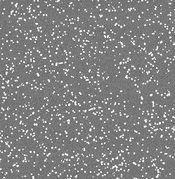
A 30 sec exposure image, CCD in front of a Fe55 source

In the dialog form, enter the window to be processed (X1,Y1,X2,Y2). Then the readout direction (CCD output port direction left/right). The conversion factor must be known within 5% accuracy. The bias offset level as also to be provided (accurate, from overscan areas or master bias frame). Select more than one image is recommended for better accuracy, as so as to enter more than 2 lines for each packet. Those packet are used to bin the histogram of a line/column N times.

Results

Console output:
Load image: iron-1.cpa
Load image: iron-3.cpa
Load image: iron-2.cpa
Load image: iron-4.cpa
CTEV=1.000000101
CTEH=0.999997222
Conversion factor=0.680809

Vertical CTE histogram as a printable plot (very good V.CTE)

Horizontal CTE histogram as a printable plot (H.CTE =0.999997222 )

Method used :
The software performs vertical histogram gathering N columns so as to have a better Signal to Noise measurement, it also uses more than one image to improve the measurement Then displays an image where the X axis is the counts in ADUs, Y the column number and Z the number of pixels having the given X counts. The softwarefinds the histogram peaks for every column and fits the best slope. As you can see on the image above, the slope that joins all the peak is slightly tilted to the left, showing that the 1620e- created at the end of the serial register (column 2048) are indeed less than 1620e-, thus showing a CTE not equal to 1. The software, according to the histogram peak slope can compute the HCTE.

The same method applies for the horizontal CTE, just swap the word vertical with horizontal and the word column with rows.

References section

1. Electronic imaging in Astronomy, by Ian S.McLean
2. Scientific Charge Coupled Devices, by J.Janesick
3. Optical CCD Detectors - CCD Tests and Characterization at ESO Garching
   
4. Astronomical CCD Observing and Reduction Techniques
   Ed. Steve B. Howell
5. In situ CCD testing
   

This file was updated by C.Cavadore, 17/02/2006